Convex & Optimal Rocket Landing Guidance Control
03 Jan 2021 From this
 To this
Overview
The goal of this study is to solve complex planetary soft landing problem with a defined set of states and control constraint. The real-time generation of fuel-optimal paths to a prescribed location on a planet’s surface is a challenging problem due to constraints on the fuel, control inputs and the states. This study also introduce a convexification of the control constraints that is proven to be lossless; this is required due to existence of nonconvex constraints on the control input magnitude at nonzero lower bound and a nonconvex constraint on its direction. Lossless convexification allows us to implement the algorithm on an autonomous real-time systems with powerful modern interior point method (IPM) solvers.
The trajectory optimization problems are nontrivial due to nonconvex control constraints and will be formulated as a finite-dimensional second-order cone program (SOCP) where it could be solve iteratively.
Partial List of Notations
$r$ = position
$T$ = Thrust vector (N)
$g$ = Gravity vector of planet (\(m/s^{2}\))
$m(t)$ = Mass of vehicle
$\alpha$ = Constant describing mass consumption rate
$T_1$ = Lower Thrust Bound
$T_2$ = Upper Thrust Bound
$\rho_1$ = Lower Thrust Bound
$\rho_2$ = Upper Thrust Bound
$m_{wet}$ = Total mass of vehicle including propellant
$t_f$ = Length of finite time
$x$ = Augmented state vector defined as $[r, \dot r]^T$
$r_z(t)$ = Vertical position
$r_x(t)$ = Downrange position
$\Theta_{alt}$ = Glideslope constraint
$S_j, v_j, a_j$ = Matrices, vectors, and scalars defining convex state constraints
$I_{sp}$ = Specific impulse of the rocket engine
$u$ = Control acceleration put on by the thrusters
$\Gamma$ = Slack variable required for convexification
$log$ = Natural logarithm
$\vert \vert x \vert \vert$ = Euclidian 2-norm of vector x
Introduction
Soft landing is the final phase of a planetary EDL (entry, descent, and landing) and it’s also referred to as the powered descent landing stage. In the powered descent stage, the vehicle is guided as close as possible to a prescribed location on the planet’s surface by using thrusters that provide the control authority. This phase concludes when the vehicle lands with zero velocity relative to the surface.
With the atmospheric qualities of the planet being stochastic, the position in which the descent phase must begin is uncertain. Thus, we would focus on the algorithm which maximize the divert capability of the craft by minimizing fuel consumption from initial condition to the terminal state.
The convex optimization is required because it allows real-time onboard implementation and has guaranteed convergence properties with deterministic criteria. The convex optimization framework will be posed as a finite-dimensional second-order cone program (SOCP) problem, as SOCP have low complexity and can be solved in polynomial time.
Planetary Landing with Thrust Pointing Constraints
The planetary soft landing problem searches for the thrust (control) profile $T_c$ and an accompanying translational state trajectory $x$ which guide a lander from an initial position $r_0$ and velocity $\dot r_0$ to a state of rest at prescribed target location on the planet while minimizing the fuel consumption.
When the target point is unreachable from a given initial state, a precision landing problem (or minimum landing error problem) is considered instead, with the objective to first find the closest reachable surface location to the target and second to obtain the minimum fuel state trajectory to that closest point.
We will solve our system in two dimensions (x,z), and the position and velocity vectors will be the size of $\Bbb R^2$. We assumed everything is in the surface fixed frame, thus the translational dynamics of the system are given as:
\[\begin{eqnarray}\ddot r(t) = g + \frac{T_c(t)}{m(t)}\\\dot m(t) = -\alpha \vert \vert T_c(t) \vert \vert \end{eqnarray}\]where $\ddot r(t) \in \Bbb R^2$ is acceleration of the vehicle, $g$ is the gravitional acceleration vector of the planet, $T_c(t)$ is the thrust vector, $m(t)$ is the mass of the vehicle, and $\alpha$ is a positive constant describing the fuel consumption rate.
For $nth$ identical thrusters with nominal thrust level $T$ and specific impulse $I_{sp}$, we can denote the thrust vector and fuel consumption rate as follow:
\[\begin{eqnarray}T_c = (nT\cos \phi)e\\\alpha = (I_{sp}g\cos \phi)^{-1}\end{eqnarray}\]But for simplicity, we’ll assume vehicle with one engine and cantilever angle $\phi$ of 0 degrees.
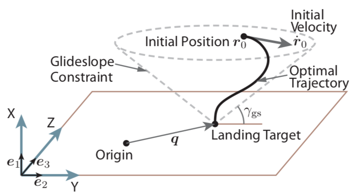 Glide Slope Constraint
The main state constraints are the glide slope constraint on the position vector and an upper bound constraint on the velocity vector magnitude.
- The glide slope constraint is described in figure above and is imposed to ensure that the lander stays at a safe distance from the ground until it reaches its target.
- Three control constraint of the thrust vector $T$
- The convex upper bound on thrust; upper bound on velocity is needed to avoid supersonic velocities for planets with atmosphere, where the control thrusters can become unreliable.
- The nonconvex lower bound on thrust; lower bound on velocity is due to the engine thrust cannot be continuously throttled down to 0
- Thrust pointing constraint; this constraint is ignored as per our simplification where only one engine is used in the vehicle.
Glide Slope Constraint
When landing on a planetary body without global positioning, terrain relative navigation is used to restrict the altitude of the vehicle to avoid vehicle crashing to the unknown terrain.
\[\begin{equation}\Theta_{alt} = \arctan \frac{r_z(t)}{r_x(t)}\end{equation}\]Additionally, it is assumed that constraints take the following affine form:
\[\begin{equation}\vert \vert S_j x(t) - v_j \vert \vert + c^T_j x(t) + a_j \leq 0\end{equation}\]where $S_j \in \Bbb R^4$, $n_j \leq 4$, $v_j \in \Bbb R^n_j$, $a_j \in \Bbb R$. Similarly, we can express the glide slope constraint like
\[\begin{equation}\vert \vert Sx \vert \vert + c^T_j x \leq 0\end{equation}\]where
\[\begin{eqnarray}S=\begin{bmatrix}1 & 0 & 0 & 0\\0 & 1 & 0 & 0\end{bmatrix}\\ c =\begin{bmatrix}-\tan\Theta_{alt} & 0 & 0 & 0\end{bmatrix}^T\end{eqnarray}\]Thrust Control Constraints
Control constraints (upper bound and lower bound) on thrust can be expressed as below:
\[\begin{equation}0 \lt T_1 \lt T(t) \lt T_2, \forall t \in [0,t_f]\end{equation}\] \[\begin{equation}\rho_1 \leq \vert \vert T(t) \vert \vert \leq \rho_2\end{equation}\] \[\begin{equation}\rho_2 \gt \rho_1 \gt 0\end{equation}\]The final time is denote as $t_f$.
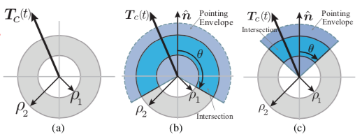 Three Control Constraints - (b) & (c) constraints are ignored since we only utilized one engine per vehicle
Initial conditions are provided as below:
$m(0)=m_{wet}$ - Total mass of the vehicle including structure, avionics, non-consummables, and fuel.
$x(0)=x_0$
$x(t_f)=0$
$x=[r, \dot r]^T$ - Constructed state of the vehicle
$r_z(t) > 0$ - Vehicle cannot travel through the ground
Problem 1 - Nonconvex Minimum Fuel Problem (thrust constraint)
Nonconvex minimum fuel problem can be summarized with the following set of equations:
\[\begin{equation}\max_{t_f,T}m(t_f) = \min_{t_f,T}\int_0^{t_f} \vert \vert T(t) \vert \vert dt \end{equation}\]Subject to: \(\begin{eqnarray}\ddot r(t) = g + \frac{T_c(t)}{m(t)}\\\dot m(t) = -\alpha \vert \vert T_c(t) \vert \vert \end{eqnarray}\)
\[\begin{eqnarray}\rho_1 \leq \vert \vert T(t) \vert \vert \leq \rho_2\\r_z(t) \leq 0\end{eqnarray}\] \[\begin{equation}\vert \vert S_j x(t) - v_j \vert \vert + c^T_j x(t) + a_j \leq 0, j=1,...,n_s\end{equation}\] \[\begin{equation}m(0)=m_{wet},r(0)=r_0,\dot r(0)=\dot {r_0},r(t_f)=\dot r(t_f)=0\end{equation}\]Problem 2 - Convexification of Problem 1
\[\begin{equation}\min_{t_f,T,\Gamma}\int_0^{t_f} \vert \vert \Gamma(t) \vert \vert dt \end{equation}\]Subject to: \(\begin{eqnarray}\ddot r(t) = g + \frac{T_c(t)}{m(t)}\\\dot m(t) = -\alpha \vert \vert T_c(t) \vert \vert \\ \vert \vert T(t) \vert \vert \leq \Gamma (t)\\ \rho_1 \leq \vert \vert \Gamma (t) \vert \vert \leq \rho_2\\r_z(t) \leq 0\\ \vert \vert S_j x(t) - v_j \vert \vert + c^T_j x(t) + a_j \leq 0, j=1,...,n_s\\ m(0)=m_{wet},r(0)=r_0,\dot r(0)=\dot {r_0},r(t_f)=\dot r(t_f)=0\end{eqnarray}\)
$\Gamma$ was introduced as a slack variable and replaces $\vert \vert T \vert \vert$ with an additional constraint $\vert \vert T(t) \vert \vert \leq \Gamma (t)$. According to this paper, the optimal solution to Problem 2 is also a feasible solution of Problem 1. This is done using the Hamiltonian of Problem 2 and using necessary conditions for optimality, pointwise maximum principle, and the transversality condition.
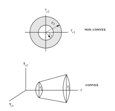 Problem 1 to Problem 2 Convexification of the Thrust Constraint
Change of Variables
Before we proceed expanding Problem 2, a change of variables is needed to allow for a much cleaner numerical algorithm. We’ll set
\[\begin{eqnarray}\sigma = \frac{\Gamma}{m}\\ u = \frac{T}{m}\end{eqnarray}\]and thus changing the translational dynamics of the system \(\begin{eqnarray}\ddot r(t) = g + u(t)\\ \frac{\dot m(t)}{m} = -\alpha \sigma (t)\\ \therefore m(t)=m_0exp[-\alpha \int_0^{t_f} \sigma (t)dt] \end{eqnarray}\)
Therefore, we must minimize the integral term in the last mass dynamical equations. The original constraints follow that \(\begin{eqnarray}\vert \vert u(t) \vert \vert \leq \sigma (t), \forall t \in [0,t_f]\\ \frac{\rho_1}{m(t)} \leq \sigma (t) \leq \frac{\rho_2}{m(t)}, \forall t \in [0,t_f]\end{eqnarray}\)
This inequality now describes a convex set. However, when we consider $m$ by itself to be variable of the problem, these inequalities become bilinear and do not define a convex region. We’ll now introduce $z$ to resolve this issue and convexify these inequalities. Let’s define $z = log m$, and then the mass depletion rate now becomes $\dot z(t) = -\alpha \sigma (t)$. The inequalities now become
\[\begin{equation}\rho_1 exp(-z(t)) \leq \sigma (t) \leq \rho_2 exp(-z(t)), \forall t \in [0,t_f] \label{inequality_1} \end{equation}\]The left side of the inequality in eqn.\ref{inequality_1} defines a convex feasible region, but the right part doesn’t. We’ll use Taylor expansion of the exponential to achieve second-order cone and linear approximation to be used in our problem. The first part of eqn.\ref{inequality_1} can be approximate by the first three terms of the series, or second-order cone:
\[\begin{equation}\rho_1 exp(-z_0)[1-(z-z_0)+\frac{(z-z_0)^2}{2}] \leq \sigma \end{equation}\]Where $z_0$ is a given constant. The right side of eqn.\ref{inequality_1} can be linear or the first two terms of the Taylor expansion. Therefore
\[\begin{eqnarray}\sigma \leq \rho_2 exp(-z_0)[1-(z-z_0)]\\ \mu_1 = \rho_1 exp(-z_0)=\frac{\rho_1}{exp(z_0)}, \mu_2 = \rho_2 exp(-z_0)=\frac{\rho_2}{exp(z_0)}\end{eqnarray}\]We now have a second order cone formulation where $z_0(t) = log(m_{wet}-\alpha \rho_2 t)$ where $z_0(t)$ serves as a lower bound on $z(t)$ at each time. We must now ensure that $z(t)$ is constrained properly with
\[\begin{eqnarray}log(m_{wet}-\alpha \rho_2 t) \leq z(t) \leq log(m_{wet}-\alpha \rho_1 t)\end{eqnarray}\]Problem 3 - Simplification with Glide Slope Constraint
\[\begin{eqnarray}\min_{t_f,u,\sigma} \int_0^{t_f} \sigma (t)dt\end{eqnarray}\]Subject to: \(\begin{eqnarray}\ddot r(t) = g + u(t)\\\dot z(t)=-\alpha \sigma (t)\\ \vert \vert u(t) \vert \vert \leq \sigma (t)\\ u_1(t)[1-(z-z_0)+\frac{(z-z_0)^2}{2}] \leq \sigma \leq u_2(t)[1-(z-z_0)]\\ log(m_{wet}-\alpha \rho_2 t) \leq z(t) \leq log(m_{wet}-\alpha \rho_1 t)\\ \vert \vert r_x(t) \vert \vert \leq \beta r_z(t)\\ m(0)=m_{wet},r(0)=r_0,\dot r(0)=\dot {r_0},r(t_f)=\dot r(t_f)=0\end{eqnarray}\)
We have replaced the general affine constraint form with the glide sloep constraint; where $\beta$ is the defined slope.
Problem 4 - Discretization of Problem 3 into Piecewise Linear Function.
For $\Delta t \gt 0$, and for each instance $t_k = k \Delta t,\forall k = 0,…,N$, we replace the continuous time with
\[\begin{eqnarray}u(t) = u_k + (u_{k+1}-u_k)t\\\sigma (t) = \sigma_k + (\sigma_{k+1} - \sigma_k)t\end{eqnarray}\]where \(\begin{equation}t=\frac{t-t_k}{\Delta t},\forall t \in [t_k,t_{k+1}),k=0,...,N-1 \end{equation}\)
Thus \(\begin{equation}\min_{u_0,...,u_N,\sigma_0,...,\sigma_N} -z_n\end{equation}\)
Subject to: for $k=0,…,N$ \(\begin{eqnarray}r_{k+1}=r_k + \frac{\Delta t}{2}(\dot r_k + \dot r_{k+1})+\frac{\Delta t^2}{12}(u_{k+1}-u_k)\\ \dot r_{k+1} = \dot r_k + \frac{\Delta t}{2}(u_k + u_{k+1})-g\Delta t\\ z_{k+1}=z_k-\frac{\alpha \Delta t}{2}(\sigma_k + \sigma_{k+1})\\ \vert \vert u_k \vert \vert \leq \sigma_k\\ u_{1,k}(t)[1-(z_k-z_{0,k})+\frac{(z_k-z_{0,k})^2}{2}] \leq \sigma \leq u_{2,k}(t)[1-(z_k-z_{0,k})]\\ log(m_{wet}-\alpha \rho_2 k \Delta t) \leq z_k \leq log(m_{wet}-\alpha \rho_1 k \Delta t)\\ \vert \vert r_x(t) \vert \vert \leq \beta r_z(t)\\ m(0)=m_{wet},r(0)=r_0,\dot r(0)=\dot {r_0},r(t_f)=\dot r(t_f)=0\\ z_0=log(m_{wet}),N\Delta t=t_f\end{eqnarray}\)
We now have general lossless-convexified algorithm and can use vehicle parameters to generate trajectories.
MATLAB Simulation
Above are the vehicle initial parameters and conditions set up through MATLAB. The specific impulse $I_{sp}$ was chosen to reflect an ethanol liquid oxygen (LOX) rocket engine performance. For this simulation, we’ll use open source solver CVX SeDuMi to solve our SOCP problem. Discretized problem 4 equations and constraints are formulated in MATLAB as per below
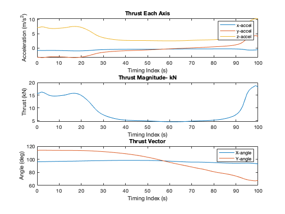
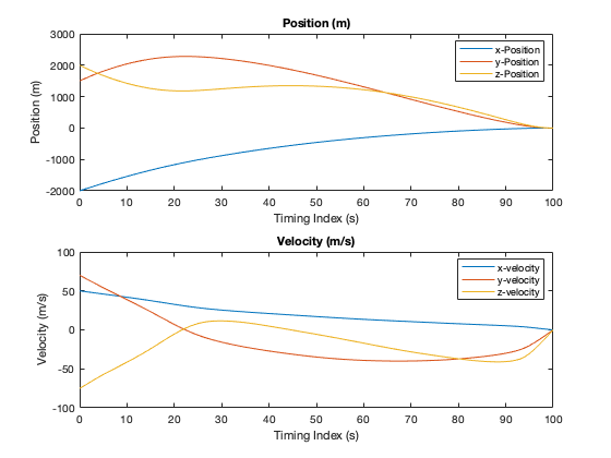
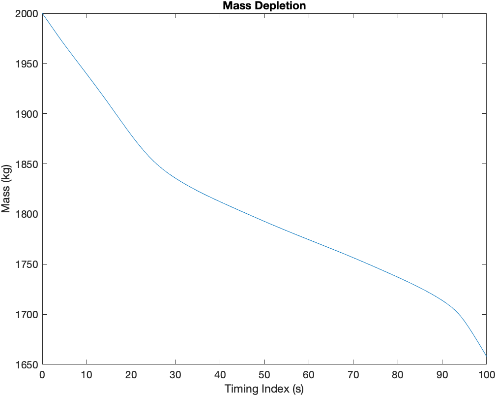
The trajectory in figure below shows how the vehicle overshot the target during the entry phase and how it works its way back towards the landing site. Keep in mind that the $t_f$ in this situation is static at 100 seconds and is not necessarily globally optimal.
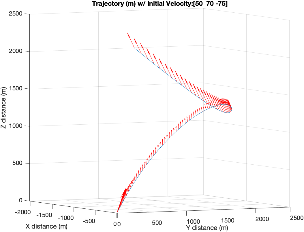
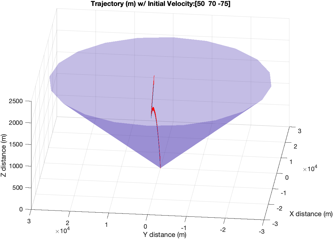 Trajectory with Glide Slope Constraint